
PerformStars · Research & Engineering
How difficult is a pool shot?
The geometry behind the score
A made ball tells us the outcome. The space available for an aiming error tells us something about the task. Here is how we turn a table position into a geometric difficulty score—and enough mathematics to reproduce it.
w is the full allowable range of cue-ball directions, in radians.
A smaller window produces a larger score. There is no upper cap.
1. A shot has a window, not just an aiming line
Imagine two shots that both finish in the same pocket. In one, the cue ball is close to a straight object ball. In the other, the contact is thin and the object ball has a long way to travel. Both pots count as one successful shot, but the permitted error in the initial cue-ball direction can be very different.
The useful question is: over what range of initial directions would the geometry still allow the pot? A pocket has a finite opening. A ball has a finite radius. Those dimensions define a range of outgoing object-ball directions. The collision then maps that range back to a range of cue-ball directions.
This is possible without learning a player's accuracy. We are measuring a property of a specified position under a specified geometric model. Player skill, execution consistency, and the outcome remain separate observations.
Our reference unit is an aiming half-window of 0.05 radians. A half-window of 0.005 radians gives D = 10; 0.0005 radians gives D = 100. Equivalently, using the full window w, the score is 0.10/w. Before rounding, doubling the score means halving the allowable window.
2. What we collect from a recording
The detector does not predict the difficulty score. It supplies observations from which we reconstruct the position. The video pipeline is described in our article on ball detection and trajectory reconstruction.
- Locate the playing surface. Table calibration maps perspective-distorted image coordinates into a rectangle attached to the playing field.
- Detect and track the balls. Frame-indexed detections establish the cue-ball track, the candidate object ball, and their starting coordinates. The current calculation uses each track's first available point.
- Identify a pocket attempt. Observed approaches to pocket regions provide candidate pockets. The selected ball, pocket, and contact geometry must support a feasible direct pot. A geometric score alone does not prove what the player intended.
- Apply physical dimensions. The discipline supplies the ball radius and nominal pocket widths. The table dimensions convert the normalized positions into metres.
- Calculate, then store. The geometric model returns the cue-ball window and score. The selected score is rounded to two decimal places when stored with the shot.
Here ℓ and b are the playing-field length and width, and (xₚ, yₚ) belongs to the normalized 1280 × 640 table rectangle—not to the original camera image. The two axes are scaled independently. Pocket widths and ball diameters stay fixed when the table size changes.
Some quantities, such as a sharply changing score near a tangential contact, are sensitive to coordinate error. Reporting two decimal places is a storage convention; it does not imply that the video measured the position with that level of physical certainty.
3. The complete geometry of a direct pot
We consider two equal-radius balls moving in a plane. The object ball initially rests at O; the cue ball starts at C. Under the ideal first-contact assumption, the object ball leaves along the line joining the centres at contact. The selected pocket is represented by a straight entrance segment. All lengths below use one consistent unit; all angles in the computation are in radians.
| Symbol | Meaning |
|---|---|
| C, O; R | Initial cue-ball centre, object-ball centre, and common ball radius |
| L = |O − C| | Initial centre-to-centre separation; the model requires L > 2R |
| P; 2a | Midpoint of the pocket entrance and its full mouth width |
| n; t = (−nᵧ, nₓ) | Outward unit mouth normal and its perpendicular unit tangent |
| x; h; d | Lateral offset, perpendicular distance, and distance from O to P |
| φ₋, φ₊; W | Feasible object-ball directions relative to n, and their full width |
| γ; β | Object-ball and cue-ball directions relative to the initial axis C → O |
| w; D | Full cue-ball aiming window and the resulting difficulty score |
3.1. Put the pocket in its own coordinate system
For a side pocket, the entrance lies along the cushion. For a corner pocket, we place a diagonal entrance between the two adjacent cushions. If V is the corner vertex and n points outward along the corner bisector, P = V − an. The two jaw tips P ± at then lie on the neighbouring cushion lines. The pocket ID still refers to that table corner; P is the centre of its entrance rather than the corner vertex.
Internally, the implementation divides every length by R, so the normalized ball radius becomes one. This changes numerical scale, not the geometry. Expressing the same inputs in millimetres instead of metres leaves the score unchanged.
3.2. Find the object ball's pocket window
Take x ≥ 0 first. A successful ideal path brings the ball centre to the mouth line before the ball touches either jaw. The segment ends at that line: we do not simulate the ball's subsequent travel down the pocket throat. Require h > 0 and a > R, and define q = √((x − a)² + h²). If q < R, the starting ball overlaps the nearer jaw and the input is rejected.
The lower boundary has two regimes. When x > a − R, the limiting path is tangent to the nearer jaw before crossing the entrance. Otherwise, the limiting clearance occurs at the entrance line itself:
Both expressions meet continuously at x = a − R, where φ₋ = 0. For negative x, first calculate the interval at |x|, then reflect it:
If φ₊ ≤ φ₋, there is no positive-width window. A position without a feasible interval returns no score. It is not assigned an arbitrary maximum difficulty.
For the symmetric case x = 0, the result reduces to:
These boundaries develop the finite-path geometry in Georgy Maurakh's Assessment of the Difficulty of a Billiard Shot (April 2025). We use the boundaries directly. The shortened denominator printed in equation (6) of that work does not follow from the difference-of-arctangents identity. For completeness, the correct expression, with x = d sinφ and h = d cosφ, is:
Throughout this article, atan2(y, x) denotes the two-argument arctangent. Keeping both arguments preserves the quadrant; using atan(y/x) can select the wrong branch for a wide interval.
3.3. Check whether the cue ball can produce those directions
A pocket can accept an outgoing direction that the starting cue-ball position cannot generate through a first contact. Let e = (O − C)/L, and let u be a desired object-ball direction. The cue ball's centre at the corresponding contact—the ghost-ball centre—is:
This approaching-contact condition matters especially when the balls are close. Merely checking that the direction is less than 90° from the initial line of centres is insufficient.
Here γ is measured from e. Choose the equivalent angular interval using k = −1, 0, or 1; retain a positive-width intersection. Contact exactly at the endpoint is interpreted as a limit. If no intersection exists, the direct pot is geometrically infeasible under this model.
3.4. Transfer the window back to the cue ball
In the frame aligned with C → O, the vector G − C has components (L − 2R cosγ, −2R sinγ). The required initial cue-ball direction is therefore:
Within the approaching-contact interval, this mapping is monotone decreasing:
We can therefore map the two boundaries instead of sampling every possible direction. The complete direct-pot score is:
The factor 0.10 sets the numerical scale. It is not fitted to a player's potting percentage. Unlike a probability, the score has no natural upper bound. A full window of 0.01° gives D ≈ 572.96; a ten-times narrower one gives D ≈ 5729.58. New calculations are no longer clipped at 200.
The local error-amplification factor follows from the same derivative:
For a narrow interval where A varies little, w is approximately the reachable object-ball window divided by A. The implementation uses the exact endpoint mapping, which also handles wide windows and intervals near the contact limit.
4. See the position, then check the calculation
The first three positions are constructed examples. The last three use archived coordinates from recorded pool positions, with their selected pocket held fixed. All six scores below were recalculated with the current uncapped model. They are illustrations, not a representative benchmark or independently verified player ratings.
Each diagram shows only the two modelled balls. Blue is the cue-ball path to contact; orange is the calculated object-ball path at the midpoint of the reachable contact interval. These are model paths, not a claim about the exact trajectory played in the recording.
A short, straight pool shot
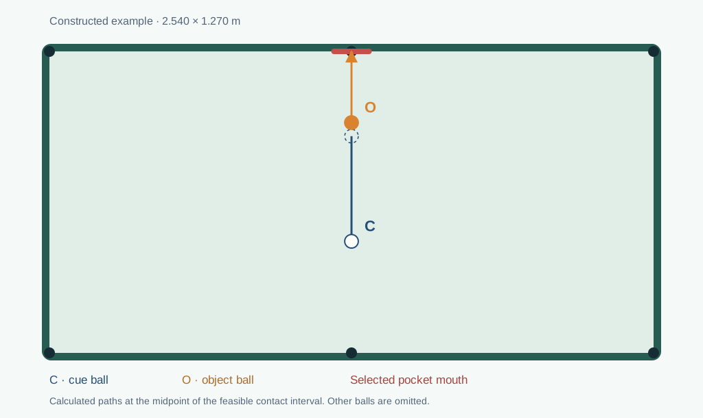
The pocket and the first-contact windows are symmetric. Both sides of the straight shot count toward the cue-ball tolerance.
- Cue → object, L
- 0.5000 m
- Object → mouth, d
- 0.3000 m
- Pocket window, W
- 0.29794289 rad
- Cue-ball window, w
- 0.0382482723 rad
D = 0.10 / 0.0382482723 ≈ 2.61Use the unrounded input data to reproduce the final decimal places.Coordinates and intermediate angles
Metres: C = (1.27000000, 0.80000000); O = (1.27000000, 0.30000000); P = (1.27000000, 0.00000000). Ball radius R = 0.028575 m; mouth width 2a = 0.147200 m.
x = 0.00000000 m; h = 0.30000000 m; δ = 0.000000000 rad.
φ₋ = -0.148971446; φ₊ = 0.148971446 rad.
γ₋ = -0.148971446; γ₊ = 0.148971446 rad.
β(γ₋) = 0.0191241362; β(γ₊) = -0.0191241362 rad.
Same pocket, same distances, a thinner cut
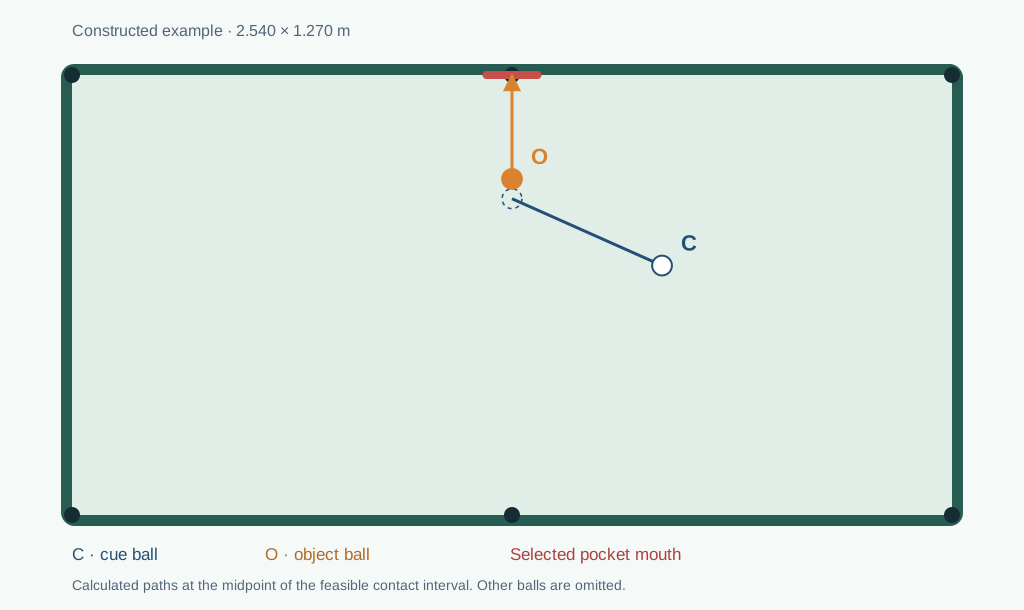
The object ball has the same pocket window as in the first diagram. The thinner contact compresses the corresponding cue-ball window.
- Cue → object, L
- 0.5000 m
- Object → mouth, d
- 0.3000 m
- Pocket window, W
- 0.29794289 rad
- Cue-ball window, w
- 0.0145960140 rad
D = 0.10 / 0.0145960140 ≈ 6.85Use the unrounded input data to reproduce the final decimal places.Coordinates and intermediate angles
Metres: C = (1.70301270, 0.55000000); O = (1.27000000, 0.30000000); P = (1.27000000, 0.00000000). Ball radius R = 0.028575 m; mouth width 2a = 0.147200 m.
x = 0.00000000 m; h = 0.30000000 m; δ = 1.047197551 rad.
φ₋ = -0.148971446; φ₊ = 0.148971446 rad.
γ₋ = 0.898226105; γ₊ = 1.196168997 rad.
β(γ₋) = -0.0959671461; β(γ₊) = -0.1105631601 rad.
The same metric position with snooker equipment
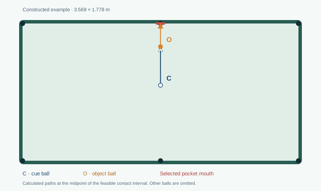
Distances remain 0.50 m and 0.30 m. A 52.5 mm ball and a nominal 90 mm entrance leave only 18.75 mm of clearance per side. The same geometric formula produces the score; there is no separate snooker multiplier.
- Cue → object, L
- 0.5000 m
- Object → mouth, d
- 0.3000 m
- Pocket window, W
- 0.12483762 rad
- Cue-ball window, w
- 0.0146326417 rad
D = 0.10 / 0.0146326417 ≈ 6.83Use the unrounded input data to reproduce the final decimal places.Coordinates and intermediate angles
Metres: C = (1.78450000, 0.80000000); O = (1.78450000, 0.30000000); P = (1.78450000, 0.00000000). Ball radius R = 0.026250 m; mouth width 2a = 0.090000 m.
x = 0.00000000 m; h = 0.30000000 m; δ = 0.000000000 rad.
φ₋ = -0.062418810; φ₊ = 0.062418810 rad.
γ₋ = -0.062418810; γ₊ = 0.062418810 rad.
β(γ₋) = 0.0073163208; β(γ₊) = -0.0073163208 rad.
A recorded side-pocket cut
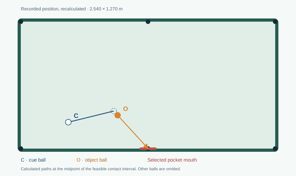
The half-window is about 0.224 degrees. The score comes from the reconstructed position, not from whether the player made the shot.
- Cue → object, L
- 0.4970 m
- Object → mouth, d
- 0.4509 m
- Pocket window, W
- 0.13321467 rad
- Cue-ball window, w
- 0.0078096331 rad
D = 0.10 / 0.0078096331 ≈ 12.80Use the unrounded input data to reproduce the final decimal places.Coordinates and intermediate angles
Metres: C = (0.47426563, 1.00607812); O = (0.96639062, 0.93662500); P = (1.27000000, 1.27000000). Ball radius R = 0.028575 m; mouth width 2a = 0.147200 m.
x = -0.30360937 m; h = 0.33337500 m; δ = 1.710999425 rad.
φ₋ = -0.807768574; φ₊ = -0.674553906 rad.
γ₋ = 0.903230851; γ₊ = 1.036445519 rad.
β(γ₋) = -0.0969214901; β(γ₊) = -0.1047311233 rad.
A recorded shot with a long cue-ball approach
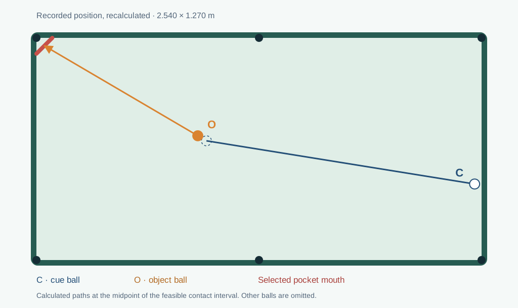
A modest cut can still demand a narrow aiming window when the cue ball starts a long way from the contact point.
- Cue → object, L
- 1.6035 m
- Object → mouth, d
- 1.0154 m
- Pocket window, W
- 0.06682291 rad
- Cue-ball window, w
- 0.0022954808 rad
D = 0.10 / 0.0022954808 ≈ 43.56Use the unrounded input data to reproduce the final decimal places.Coordinates and intermediate angles
Metres: C = (2.50031250, 0.83542187); O = (0.92075000, 0.55959375); P = (0.04525483, 0.04525483). Ball radius R = 0.028575 m; mouth width 2a = 0.128000 m.
x = -0.25537603 m; h = 0.98276110 m; δ = 0.612518206 rad.
φ₋ = -0.287692988; φ₊ = -0.220870079 rad.
γ₋ = 0.324825218; γ₊ = 0.391648127 rad.
β(γ₋) = -0.0117718651; β(γ₊) = -0.0140673459 rad.
A recorded position beyond the old 200 ceiling
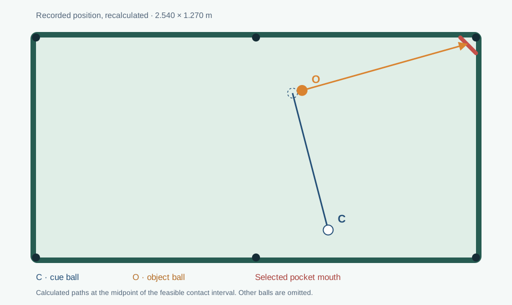
Only part of the pocket window is reachable by a first contact. The result is a very narrow cue-ball window and a score well above 200. This illustrates sensitivity near a tangential contact, not a verified rating of the player.
- Cue → object, L
- 0.8197 m
- Object → mouth, d
- 0.9936 m
- Pocket window, W
- 0.05839908 rad
- Cue-ball window, w
- 0.0000513989 rad
D = 0.10 / 0.0000513989 ≈ 1945.57Use the unrounded input data to reproduce the final decimal places.Coordinates and intermediate angles
Metres: C = (1.68671875, 1.11125000); O = (1.53590625, 0.30559375); P = (2.49474517, 0.04525483). Ball radius R = 0.028575 m; mouth width 2a = 0.128000 m.
x = 0.49391409 m; h = 0.86208891 m; δ = 0.970448671 rad.
φ₋ = 0.492264885; φ₊ = 0.550663965 rad.
γ₋ = 1.462713556; γ₊ = 1.501014840 rad.
β(γ₋) = -0.0697300883; β(γ₊) = -0.0697814872 rad.
The recorded examples come from two processing runs of a local video archive and may contain related observations. Initial coordinates use the first available point of each track, which need not come from the same frame. Reconstruction errors and pocket selection remain sources of uncertainty, particularly in the final near-tangential example.
5. One geometric model, different equipment
A discipline enters the calculation through physical dimensions. Snooker uses the same equations as pool, with its own ball radius, pocket widths, and table dimensions. There is no manually chosen “harder game” multiplier. The parameters used in this article are:
| Discipline | Ball diameter | Corner mouth | Side mouth |
|---|---|---|---|
| Pool | 57.15 mm | 128 mm | 147.2 mm |
| Snooker | 52.5 mm | 90 mm | 90 mm |
The simplified mouth widths are model parameters, not universal specifications for every manufactured table. In particular, 90 mm is our nominal straight-entry approximation for snooker, not a universal pocket-width requirement. We retain separate corner and side settings even when their configured values are equal. Curved jaws and the throat behind the entrance are not modelled.
Pool table dimensions vary with table size. The current snooker configuration uses a full-size 3.569 × 1.778 m playing field and a 52.5 mm ball. The WPBSA equipment rules specify the playing area and ball diameter; those values should not be confused with our simplified 90 mm pocket setting.
A smaller snooker ball changes the contact mapping and leaves more space within a given opening. Its smaller pocket changes the window in the opposite direction. Both effects enter the equations explicitly through R and a. Example 3 holds the distances fixed, so its difference from example 1 comes from equipment dimensions rather than a longer table. At corresponding fractional table positions, the larger snooker playing field also increases the physical distances.
In the straight examples above, pool gives D ≈ 2.61 and snooker D ≈ 6.83 at the same 0.50 m cue-to-object and 0.30 m object-to-mouth distances. This comparison belongs to that position and those configured mouth widths; it is not a universal ratio between the two games.
Equal scores across disciplines mean equal cue-ball angular windows within these assumptions. Differences in real jaw shape, required pace, or stroke technique are outside this comparison.
6. Why smaller pockets matter: snooker and Heyball
The useful quantity is not the pocket opening alone, but the space remaining for the ball's centre. For a straight entry, the available clearance on each side is:
With the configured snooker dimensions, m = (90 − 52.5)/2 = 18.75 mm. The configured pool side pocket leaves (147.2 − 57.15)/2 = 45.025 mm. At the same object-to-mouth distance, the smaller snooker clearance produces a narrower pocket window. We then use the actual ball radius again in the contact mapping to obtain the cue-ball window and score.
| Equipment | Mouth width | Ball diameter | Clearance m |
|---|---|---|---|
| Pool corner — configured | 128 mm | 57.15 mm | 35.425 mm |
| Pool side — configured | 147.2 mm | 57.15 mm | 45.025 mm |
| Snooker — configured approximation | 90 mm | 52.5 mm | 18.750 mm |
| Heyball corner — BOJUE example | 85 mm | about 57.2 mm | about 13.9 mm |
| Heyball side — BOJUE example | 82 mm | about 57.2 mm | about 12.4 mm |
Heyball illustrates why a pool-sized ball does not imply a pool-sized target. BOJUE documents an 85 mm corner / 82 mm side configuration for one tournament-focused setup, and also describes wider alternatives. These are manufacturer-specific examples, not a single universal Heyball standard. Measurements must use comparable jaw reference points.
Current implementation status: the shared equipment helper has no dedicated Heyball profile. Passing 'heyball' to the high-level helper currently falls back to pool defaults, which is not a calibrated Heyball calculation. The manufacturer dimensions above have not been installed as a production profile.
The underlying formula can already evaluate explicit physical dimensions. A caller with a measured mouth can use the lower-level function directly, supplying C, O, the entrance centre P, and its outward normal n in a consistent coordinate system. For example, the following uses the manufacturer's approximate ball diameter and 85 mm corner opening:
import { difficalty } from './model.mjs';

// All positions and sizes are in metres.
// P is the entrance midpoint, not the table corner vertex.
const result = difficalty(C, O, P, 0.0572 / 2, 0.085, {
  normal: n
});
For an 82 mm side entrance, use 0.082 m and the corresponding side-pocket centre and normal. This is an explicit equipment calculation, not support for every Heyball table. The model still omits the rounded jaw profile for both snooker and Heyball, as well as the dynamics of a ball touching those jaws.
7. Where we use this in PerformStars
Difficulty adds context to the shot record. A coach can inspect the position, the outcome, and the geometric demand together, instead of treating every pot or miss as the same task.
| Where | How the score is used |
|---|---|
| Individual shot review | The shot detail view displays the stored score as “Make difficulty” alongside the diagram and other metrics. |
| Workout summaries | The current aggregation counts shots with a score above 18 as complex shots, where a finite estimate is available. |
| Coaching reports | The report pipeline groups scored attempts into difficulty buckets and can examine made/miss counts within those groups. |
| Spreadsheet exports | The score is exported as Pocket complexity, allowing a coach or researcher to inspect the underlying shot records. |
The present default report thresholds are easy ≤ 12, medium > 12 and ≤ 18, and hard > 18. These are configurable product groupings, not boundaries derived from geometry. The full numerical score retains more information than the group name.
We keep the distinction between a geometric input and an observed outcome. A high score does not certify a good stroke; a low score does not make a miss impossible. The value helps organize review, locate demanding attempts, and ask more specific coaching questions.
Historical records were not rewritten when the model changed. In particular, an old stored value of 200 can reflect the earlier cap, whereas current calculations are uncapped. Recalculate the same inputs with the same model before treating scores from different generations as directly comparable.
8. What the model leaves open
The model evaluates a direct first contact and a straight finite path to an idealized entrance. It does not model collisions with other balls, cushion-first routes, banks, jaw rebounds, pocket depth, cloth friction, speed, spin, cue access near a rail, or position for the next shot. Passing the model's entrance criterion is not a simulation of the complete physical pocketing event.
Nor should every distance experiment be forced to be monotone. At a fixed oblique angle toward a pocket centre, increasing distance can first open a window previously blocked by the near jaw, then narrow it as the pocket becomes angularly smaller. The strict relationship is between the score and the calculated cue-ball window: a smaller positive w gives a larger D.
The published formula makes these assumptions inspectable. It lets another researcher check the arithmetic, vary the nominal equipment dimensions, and identify a disagreement with the geometry instead of having to infer the meaning of a black-box score.
9. Reproduce the numbers
We provide a snapshot of the actual shared scoring code used to generate this article, its equipment configuration, and full-precision example inputs. This article and its example runner use the direct-pot calculation for pool and snooker. No model weights, player history, database connection, or external package is required to run it.
Save all four files in the same folder and run the example runner with Node.js:
node verify.mjsIt prints the difficulty and full cue-ball window for each illustration. To calculate another position, import difficultyFromTablePoints, pass the cue and object coordinates in the normalized 1280 × 640 rectangle, the pocket ID, table size, and discipline ('pool' or 'snooker' for this article). Pocket IDs are 0 top-left, 1 top-middle, 2 top-right, 3 bottom-right, 4 bottom-middle, and 5 bottom-left.
import { difficultyFromTablePoints } from './model.mjs';

// 9-foot pool: physical field 2.54 × 1.27 m.
// C = (1.27, 0.80) m; O = (1.27, 0.30) m.
const result = difficultyFromTablePoints(
  { x: 640, y: 0.80 * 640 / 1.27 },
  { x: 640, y: 0.30 * 640 / 1.27 },
  1, 9, 'pool'
);

console.log(result.compl.toFixed(2)); // 2.61
console.log(result.cueAngularTolerance); // radians
Reference snapshot: 2026-11-03. Scoring-source SHA-256: b1d01303fe03316068677c8b921f131a0b5a26bf5d3be3b3800baf6b4e0faadf. The digest identifies the original server source before its import path was adjusted for this standalone download.
Background and provenance
Georgy Maurakh, Assessment of the Difficulty of a Billiard Shot, April 2025, provided the pocket-window starting point. The contact construction, branch handling, uncapped score, and published examples describe the PerformStars implementation as of this article's date. The archived recorded coordinates were recalculated locally; the examples do not establish empirical player-performance claims.
Continue reading: Teaching a Computer to Understand Billiards · Shot statistics.